timeseries usage
The timeseries augmentation functions in niacin fall into two broad categories: transforms which occur in the time domain, and transforms which occur in the frequency domain. Basically, this means the first category operates on the recorded values as elements in a sequence, and the second category decomposes a sequence into a set of estimated frequency components, then operates on those components.
Note
niacin assumes that your timeseries data are regularly sampled. If this is not the case, you will want to transform your data such that you have equal intervals of time between each value in the series.
Time
For timeseries data, working in the time domain means that your x-axis is some unit of time like minutes or years, and your y-axis is some value of interest. Typically, this is the domain in which signals are initially recorded, like the microsecond updates in the price of a stock, or hourly recordings of temperature.
Classical timeseries data has a number of properties, like stationarity and self-similarity. If we know that our timeseries data fits those assumptions, we can generate augmented examples by doing things like reversing the order of the sequence, or by cropping sub-sequences out of the original sequence.
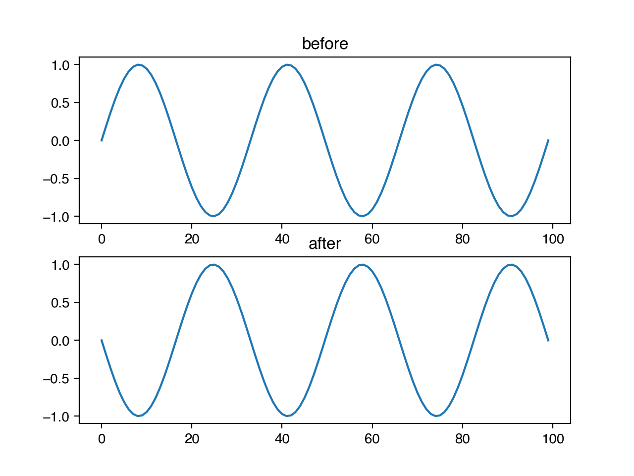
In niacin, we can reverse a sequence like this, where the parameter p refers to the probability that the transform will be applied to this sequence.
import niacin.timeseries as ts
ts.reverse(x, p=1.0)
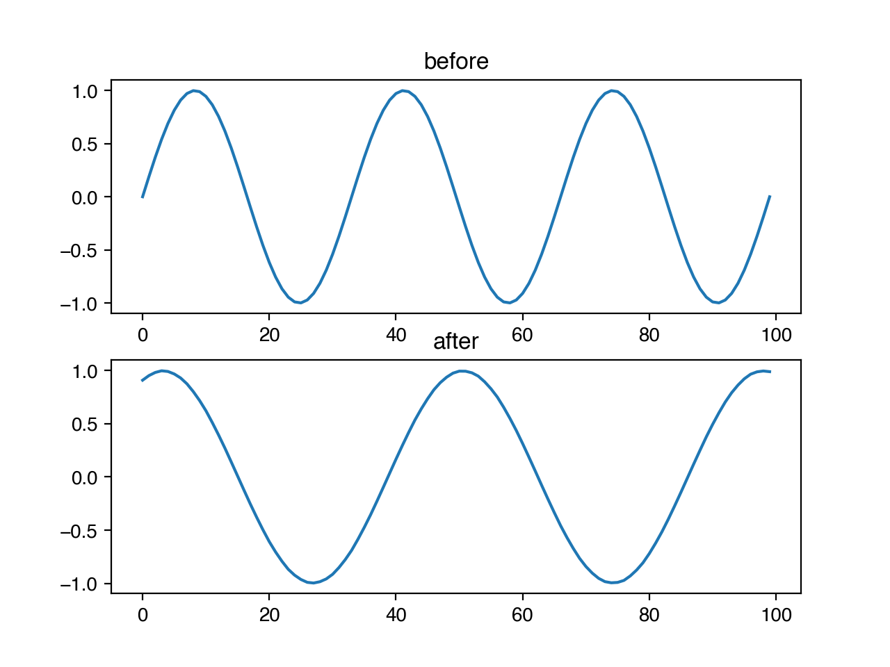
Similarly, we can use niacin to crop and re-stretch a timeseries, by providing both p, the probability that this should happen at all, and m, the magnitude of the transform if applied. For this transform specifically, the m parameter corresponds to the fraction of the original sequence removed by the cropping. Where in the sequence the crop begins is chosen randomly, uniformly across the possible starting positions.
ts.crop_and_stretch(x, 1.0, 0.3)
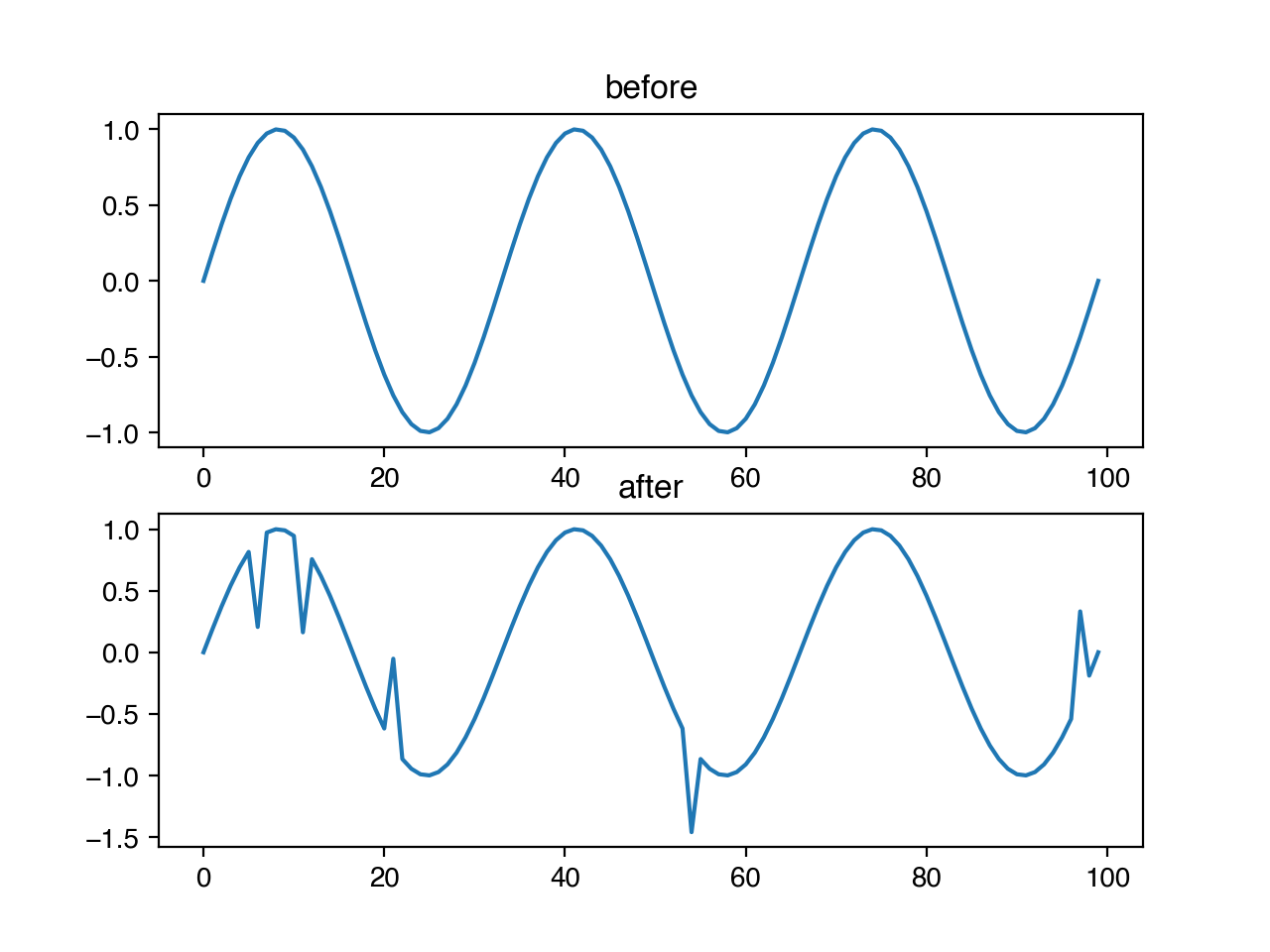
We may also wish to make our models robust to infrequent, anomalous data points. We can add spikes to our timeseries with niacin, by specifying the probability that any entry should have a spike, and the magnitude of the size of that spike as a fraction of the standard deviation of the data. The direction of the spike (positive or negative) is chosen randomly with uniform probability.
ts.add_spike(x, 0.05, 1.0)
The time-domain transformations include:
- add_slope_trend
- add_spike
- add_step_trend
- add_warp
- crop_and_stretch
- flip
- reverse
Frequency
The frequency domain represents the way signals evolve over time by decomposing them into changes that occur over individual periods. For example, here is the sine curve that we have been using, but plotted in the frequency domain.
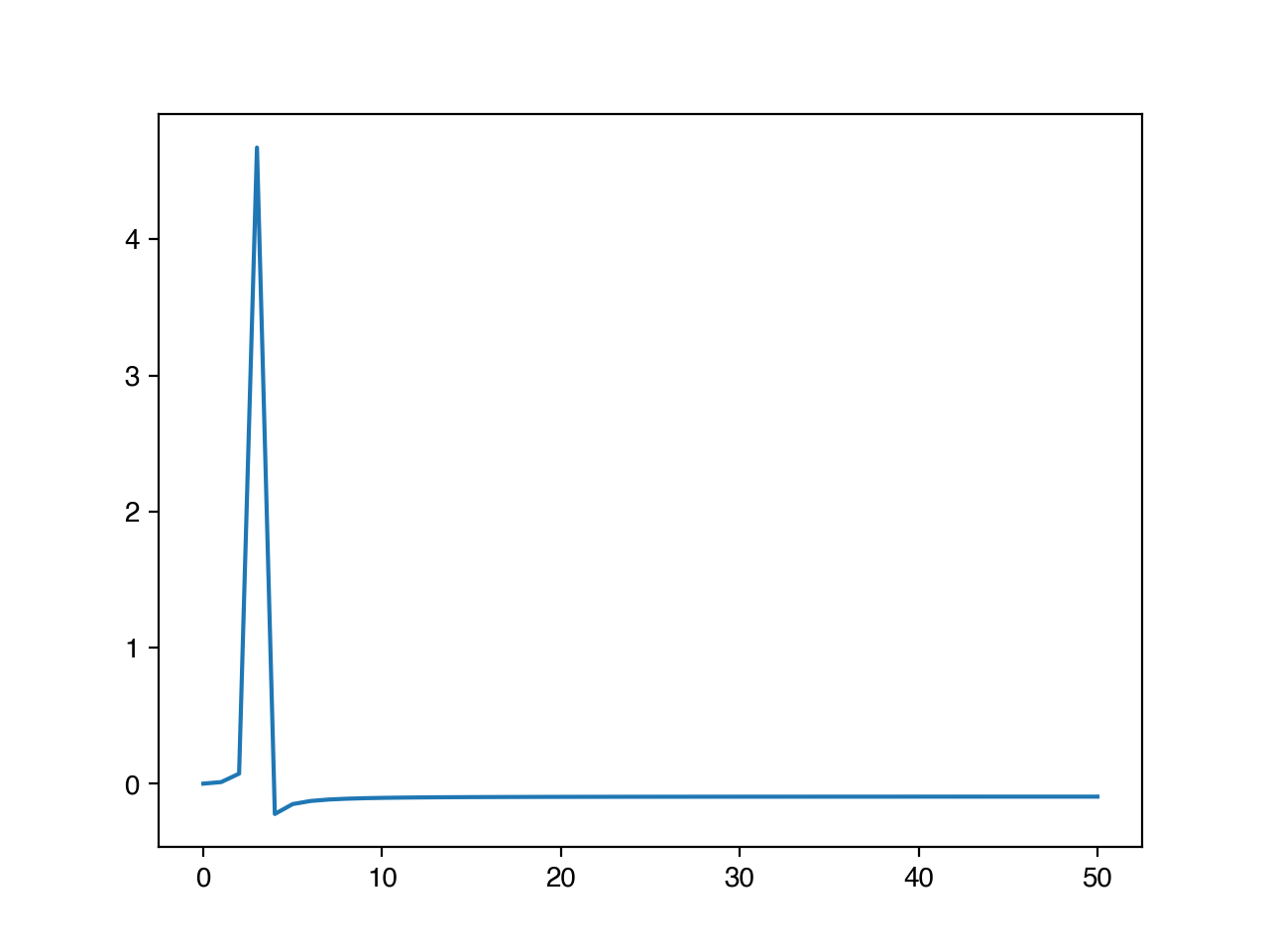
You’ll notice that there is a single large peak at 3 – this is because a full sine curve fits into our sequence 3 times. Stated another way, its frequency is 1/3.
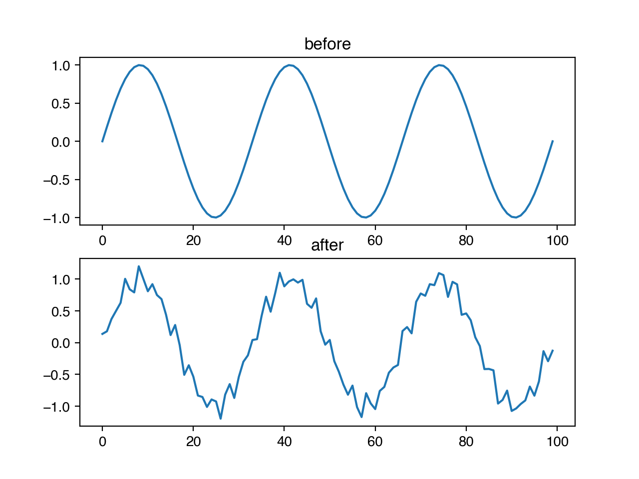
Operations like adding high frequency noise or dropping specific frequencies from a signal are easier to complete in the frequency domain. There are a number for transforms for doing things like this in niacin. For example, we might want to add small, randomly determined frequencies to our timeseries to help ensure that our algorithms are robust to periodic noise. We can do this with the random frequency noise transform, by setting p to be the probability that any frequency gets added noise, and m to be the magnitude of noise as a fraction of the amplitude of the largest frequency.
ts.add_random_frequency_noise(x, 0.1, 0.1)
The frequency-domain transformations include:
- add_discrete_phase_shift
- add_high_frequency_noise
- add_random_frequency_noise
- remove_random_frequency